---
title: "Joining / Merging Data"
---
# Relational Data
## Relational Data
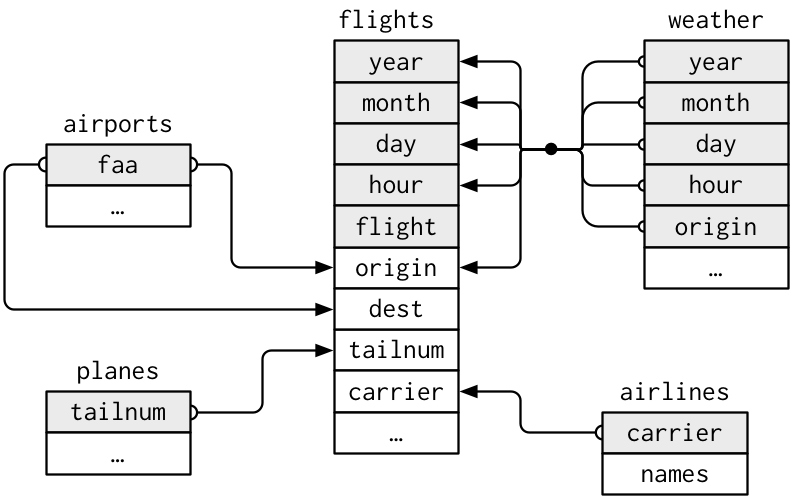
## Visualizing Relational Data
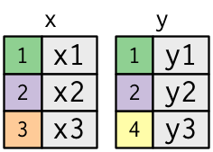
* **Primary key**: uniquely identifies an observation in its own table. For example, `planes$tailnum` is a primary key because it uniquely identifies each plane in the planes table.
* **Foreign key**: uniquely identifies an observation in another table. For example, the `flights$tailnum` is a foreign key because it appears in the flights table where it matches each flight to a unique plane.
## 3 families of verbs designed to work with relational data
* **Mutating joins**: add new variables to one data frame from matching observations in another
* **Filtering joins**: filter observations from one data frame based on whether or not they match an observation in the other table.
* **Set operations**: treat observations as if they were set elements
## Inner Join
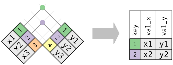
Matches pairs of observations whenever their keys are equal:
## Outer Joins
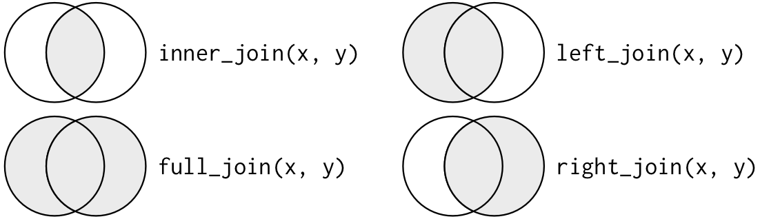
* `left_join` keeps all observations in x
* `right_join` keeps all observations in y
* `full_join` keeps all observations in x and y
## Outer Joins
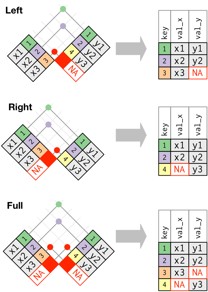 ## Outer Joins: another visualization
# Potential Problems
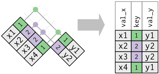
## Duplicate Keys
### One table w/ duplicates
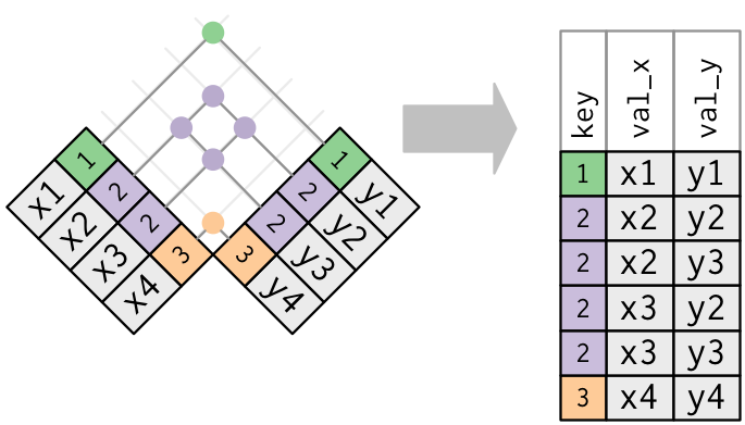
## Duplicate Keys
### Both tables w/ duplicates
## Missing Keys
### `semi_join(x, y)` keeps all observations in x that have a match in y.
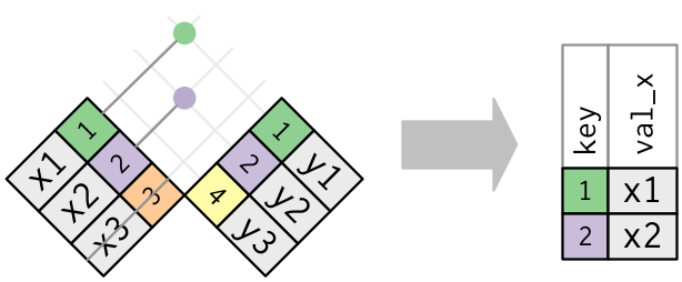
## `anti_join(x, y)` drops all observations in x that have a match in y.
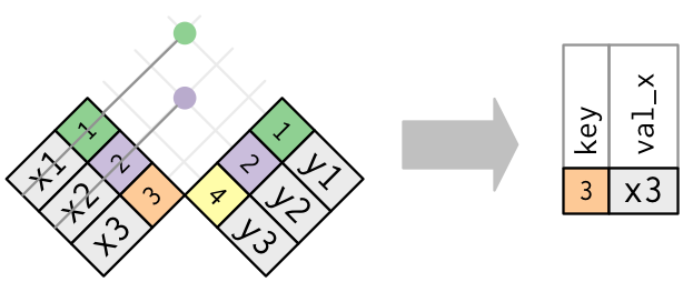
Anti-joins are useful for diagnosing join mismatches.
# Compare with other functions
## `merge()`
`base::merge()` can perform all four types of joins:
dplyr | merge
-------------------|-------------------------------------------
`inner_join(x, y)` | `merge(x, y)`
`left_join(x, y)` | `merge(x, y, all.x = TRUE)`
`right_join(x, y)` | `merge(x, y, all.y = TRUE)`
`full_join(x, y)` | `merge(x, y, all.x = TRUE, all.y = TRUE)`
* specific dplyr verbs more clearly convey the intent of your code: they are concealed in the arguments of merge().
* dplyr's joins are considerably faster and don't mess with the order of the rows.
## SQL
SQL is the inspiration for dplyr's conventions, so the translation is straightforward:
dplyr | SQL
-----------------------------|-------------------------------------------
`inner_join(x, y, by = "z")` | `SELECT * FROM x INNER JOIN y USING (z)`
`left_join(x, y, by = "z")` | `SELECT * FROM x LEFT OUTER JOIN y USING (z)`
`right_join(x, y, by = "z")` | `SELECT * FROM x RIGHT OUTER JOIN y USING (z)`
`full_join(x, y, by = "z")` | `SELECT * FROM x FULL OUTER JOIN y USING (z)`
* Note that "INNER" and "OUTER" are optional, and often omitted.
* SQL supports a wider range of join types than dplyr
## Set Operations
* `intersect(x, y)`: return only observations in both x and y.
* `union(x, y)`: return unique observations in x and y.
* `setdiff(x, y)`: return observations in x, but not in y.
## Outer Joins: another visualization

# Potential Problems
## Duplicate Keys
### One table w/ duplicates

## Duplicate Keys
### Both tables w/ duplicates

## Missing Keys
### `semi_join(x, y)` keeps all observations in x that have a match in y.

## `anti_join(x, y)` drops all observations in x that have a match in y.

Anti-joins are useful for diagnosing join mismatches.
# Compare with other functions
## `merge()`
`base::merge()` can perform all four types of joins:
dplyr | merge
-------------------|-------------------------------------------
`inner_join(x, y)` | `merge(x, y)`
`left_join(x, y)` | `merge(x, y, all.x = TRUE)`
`right_join(x, y)` | `merge(x, y, all.y = TRUE)`
`full_join(x, y)` | `merge(x, y, all.x = TRUE, all.y = TRUE)`
* specific dplyr verbs more clearly convey the intent of your code: they are concealed in the arguments of merge().
* dplyr's joins are considerably faster and don't mess with the order of the rows.
## SQL
SQL is the inspiration for dplyr's conventions, so the translation is straightforward:
dplyr | SQL
-----------------------------|-------------------------------------------
`inner_join(x, y, by = "z")` | `SELECT * FROM x INNER JOIN y USING (z)`
`left_join(x, y, by = "z")` | `SELECT * FROM x LEFT OUTER JOIN y USING (z)`
`right_join(x, y, by = "z")` | `SELECT * FROM x RIGHT OUTER JOIN y USING (z)`
`full_join(x, y, by = "z")` | `SELECT * FROM x FULL OUTER JOIN y USING (z)`
* Note that "INNER" and "OUTER" are optional, and often omitted.
* SQL supports a wider range of join types than dplyr
## Set Operations
* `intersect(x, y)`: return only observations in both x and y.
* `union(x, y)`: return unique observations in x and y.
* `setdiff(x, y)`: return observations in x, but not in y.